Operations
In the section on kernels we saw how to compile and run a simple kernel. However, working directly with kernels is not necessarily convenient:
If you always use the same kernel with the same buffers, you need to pass them all around in your code.
A kernel may be designed or optimized for a specific work-group size, but that is not captured with the kernel.
Kernels may impose alignment or padding requirements on the buffers used with them, but this is not captured programmatically.
If you use a buffer with multiple kernels, they may each have different padding or alignment requirements, and you’ll need to ensure that you pad the buffer allocation appropriately to satisfy all of them.
Some algorithms require running multiple kernels, and it would be useful to have the same interface as for single-kernel algorithms.
“Operations” are higher-level constructs that address these shortcomings. In the simplest case, an operation bundles a kernel together with information about what sort of buffers they’re used with. Each buffer requirement is called a “slot”. For example, a transpose operation might have a “src” slot which requires a 10×5 buffer of int32 and a “dest” slot which requires a 5×10 buffer of int32.
Each slot also requires a matching buffer to be bound to it. When the operation runs, it operates on the currently-bound buffers.
Operations can also be composed to build more complex algorithms from simple ones.
Let’s see an example before diving into the details:
import numpy as np

import katsdpsigproc.accel
from katsdpsigproc.accel import Dimension, IOSlot, Operation, build, roundup

SOURCE = """
<%include file="/port.mako"/>

KERNEL void multiply(GLOBAL float *data, float scale) {
    data[get_global_id(0)] *= scale;
}
"""


class Multiply(Operation):
    WGS = 32

    def __init__(self, queue, size, scale):
        super().__init__(queue)
        program = build(queue.context, "", source=SOURCE)
        self.kernel = program.get_kernel("multiply")
        self.scale = np.float32(scale)
        self.slots["data"] = IOSlot((Dimension(size, self.WGS),), np.float32)

    def _run(self):
        data = self.buffer("data")
        self.command_queue.enqueue_kernel(
            self.kernel,
            [data.buffer, self.scale],
            global_size=(roundup(data.shape[0], self.WGS),),
            local_size=(self.WGS,),
        )


ctx = katsdpsigproc.accel.create_some_context()
queue = ctx.create_command_queue()
op = Multiply(queue, 50, 3.0)
op.ensure_all_bound()
buf = op.buffer("data")
host = buf.empty_like()
host[:] = np.random.uniform(size=host.shape)
buf.set(queue, host)
op()
buf.get(queue, host)
print(host)
The kernel SOURCE is unchanged from the previous example. However, we’ve
now encapsulated all the logic for multiplying a buffer by a constant into a
class Multiply, which derives from Operation. The constructor
builds the kernel much as before; what’s new is the use of IOSlot and
Dimension. We’ll come to the details of those in the next section.
We also see that we’re no longer allocating the buffer ourselves. Instead, the
call to Operation.ensure_all_bound() takes care of allocating memory
for all the associated buffers of an operation. We could still choose to
allocate our own buffers and Operation.bind() them; this can be useful
for example if using double-buffering so that one buffer is in use by the
operation while another is busy transferring data to or from the host.
To enqueue the operation, we simply call it as a function. Because the object encapsulates all the information about how to run the operation and the buffers involved, we don’t need to provide any arguments.
Dimensions
A Dimension specifies size and padding requirements along one axis of
a (possibly) multi-dimensional array. There is a subtle but
important rule about Dimension: a specific
Dimension object always resolves to a specific padded size. Thus, if
a single object is shared between two buffers, it not only gives them the same
requirements, it constrains them to have the same amount of padding. This
can be useful as it allows a single linear address to be used for multiple
buffers. But it can also lead to unnecessarily strict constraints, so in some
cases you may wish to construct two separate but identical dimension objects
rather than re-using one object.
The most common case for a padding requirement is to compensate for a kernel’s
global_size being rounded up to a multiple of the work group size. This is
seen in the example above: Dimension(size, self.WGS) rounds size up to
a multiple of self.WGS and makes it the minimum for the padded size
(larger padded sizes are still permitted, even if not a multiple of
self.WGS). There are other options that can be specified, including to
disallow padding (to ensure the buffer is contiguous); refer to the
constructor documentation for details.
Slots
An IOSlot takes a tuple of dimensions to specify the
multi-dimensional shape of a buffer, and a dtype. For convenience, axes
without padding requirements may be specified just with an integer size
instead of a Dimension. It also has a currently-bound buffer
(initially None).
For implementation reasons relating to composing operations, the buffer bound
to a slot should be retrieved with Operation.buffer() rather than via
the slots dictionary.
Operation templates
The Multiply operation in our example is fine if we only want one of them,
but what if we want several with different sizes or scale factors? Each time
we instantiate a new one we will need to re-run the template engine and the
compiler, which is not very efficient. To avoid this overhead, it is
conventional to split out the static parts of each operation into an
“operation template” so that multiple Operation objects can share
the same program.
Let’s see how that might look in our example:
import numpy as np

import katsdpsigproc.accel
from katsdpsigproc.accel import Dimension, IOSlot, Operation, build, roundup

SOURCE = """
<%include file="/port.mako"/>

KERNEL void multiply(GLOBAL float *data, float scale) {
    data[get_global_id(0)] *= scale;
}
"""


class MultiplyTemplate:
    WGS = 32

    def __init__(self, context):
        self.program = build(context, "", source=SOURCE)

    def instantiate(self, queue, size, scale):
        return Multiply(self, queue, size, scale)


class Multiply(Operation):
    def __init__(self, template, queue, size, scale):
        super().__init__(queue)
        self.template = template
        self.kernel = template.program.get_kernel("multiply")
        self.scale = np.float32(scale)
        self.slots["data"] = IOSlot((Dimension(size, template.WGS),), np.float32)

    def _run(self):
        data = self.buffer("data")
        self.command_queue.enqueue_kernel(
            self.kernel,
            [data.buffer, self.scale],
            global_size=(roundup(data.shape[0], self.template.WGS),),
            local_size=(self.template.WGS,),
        )


ctx = katsdpsigproc.accel.create_some_context()
queue = ctx.create_command_queue()
op_template = MultiplyTemplate(ctx)
op = op_template.instantiate(queue, 50, 3.0)
op.ensure_all_bound()
buf = op.buffer("data")
host = buf.empty_like()
host[:] = np.random.uniform(size=host.shape)
buf.set(queue, host)
op()
buf.get(queue, host)
print(host)
This doesn’t use any new features of katsdpsigproc; we’ve simply refactored. There are some conventions used:
The template class has the same name as the operation class, with
Templateappended.It has an
instantiate()method which returns an instance of the operation, passing all its arguments through.The operation constructor takes the template as the first argument, and assigns it to a
templateattribute.The call to
get_kernel()is only done in the operation, not the template. This is because in PyOpenCL, two threads cannot safely call the same kernel object at the same time. With each operation having its own kernel object, it is safe for different threads to use different operations built from the same operation template.
Composing operations
It should be noted that while the operation we have shown consists of running
a single kernel, there is no requirement that this should be the case. It
would be entirely possible to compile multiple kernels and run them all in the
_run() method. You could even define your own methods to run the
kernels in different combinations.
However, bundling multiple kernels into one operation is an inflexible way of doing composition, as it doesn’t easily support recombining the kernels in different ways. In this section, we’ll instead show how to create composite operations from individual ones.
To keep the example small, we’ll use two operations provided by katsdpsigproc:
Fill, which fills an array with a constant; and HReduce,
which sums along rows of a 2D array. This is obviously not a terribly useful
combination, but it will illustrate the principles.
import numpy as np

import katsdpsigproc.accel
import katsdpsigproc.fill
import katsdpsigproc.reduce


class FillReduceTemplate:
    def __init__(self, context):
        self.fill = katsdpsigproc.fill.FillTemplate(context, np.float32, "float")
        self.hreduce = katsdpsigproc.reduce.HReduceTemplate(
            context, np.float32, "float", "a+b", "0.0f"
        )

    def instantiate(self, queue, shape):
        return FillReduce(self, queue, shape)


class FillReduce(katsdpsigproc.accel.OperationSequence):
    def __init__(self, template, queue, shape):
        self.fill = template.fill.instantiate(queue, shape)
        self.hreduce = template.hreduce.instantiate(queue, shape)
        operations = [("fill", self.fill), ("hreduce", self.hreduce)]
        compounds = {"src": ["fill:data", "hreduce:src"], "dest": ["hreduce:dest"]}
        super().__init__(queue, operations, compounds)
        self.template = template

    def __call__(self, fill_value):
        self.fill.set_value(fill_value)
        super().__call__()


ctx = katsdpsigproc.accel.create_some_context()
queue = ctx.create_command_queue()
op_template = FillReduceTemplate(ctx)
op = op_template.instantiate(queue, (10, 5))
op(42)
print(op.buffer("dest").get(queue))
This time the operation inherits from OperationSequence, which is a
subclass of Operation for composed operations. Its constructor takes
two important arguments:
A list of child operations, as
(name, operation)tuples. The default implementation of __call__ runs each of these operations in sequence (hence the class name), although nothing stops you from overriding it to provide other logic.A dictionary specifying the slots of the compound operation. Each key in this dictionary is the name of a slot of the compound operation. The value associated with the key is a list of slots on the individual operations that the compound slot corresponds to, in the form
op-name:slot. In this case we’re indicating that thedataslot on the fill operation and thesrcslot on the reduction operation must point at the same buffer, and from the outside that slot will be known assrc.Sometimes the component operations might or might not have particular slots depending on how they’re configured. For convenience, non-existent slots are silently ignored.
If a slot of a child is not listed here at all, it will be presented in the parent as
op-name:slot. It’s recommended that this is avoided as it exposes the internals of the implementation.
The real power of OperationSequence is that it resolves all the
padding requirements for the slots: any buffer bound to the src slot needs
to satisfy the requirements of both the operations to which it is bound, but
this is handled automatically.
It is also possible for the child operations to themselves be instances of
OperationSequence and thus create more and more complex operations,
ending with a top-level operation that encapsulates an entire pipeline. At
this level one may need to override the default __call__() or provide
additional methods to run individual pieces of the pipeline as needed, while
still having the benefit of linking slots together.
Aliasing scratch buffers
In more complex (particularly composed) operations, it’s not uncommon for some slots to represent internal scratch space rather than inputs or outputs. When such operations are themselves composed, this can lead to wasted memory as each operation has its own scratch space, even though they are not in use at the same time and a single scratch area could be reused. If the scratch slots have the same shape and dtype then this can be handled by connecting them to a single slot on the parent operation, but that’s not always the case.
To handle this case, the OperationSequence constructor takes an
additional dictionary for mapping slots, similar to the one already seen. The
restrictions are much weaker: the child slots that are grouped together do not
need to match in shape or dtype. The tradeoff is that the resulting slot is
not fully-fledged (it is an AliasIOSlot rather than an
IOSlot) so does not have a dtype, shape etc. It is normally not used
directly, other than to serve as a source creating further alias slots if this
operation is composed into an even higher-level one.
It is recommended that you document scratch slots of your operations (including their sizes and anything unusual about data lifetime) so that users of your operation can decide how best to alias them with other scratch slots.
Kernel fusion
It should be noted that there is another way to combine operations, which is to write a single kernel that performs all of them. For example, if you have three arrays A, B and C, and want to compute (element-wise) A×B+C, then it is much more efficient to have a single kernel that does this combined combination on each element than to run a multiply kernel followed by an add kernel. Combining kernels in this way is referred to as “kernel fusion”. Unfortunately, it is a hard problem and CUDA and OpenCL do not provide any support for it, and nor does katsdpsigproc in general.
However, see Macros for kernels for information about macros that help with writing kernels that fuse custom operations with standard ones like transposition.
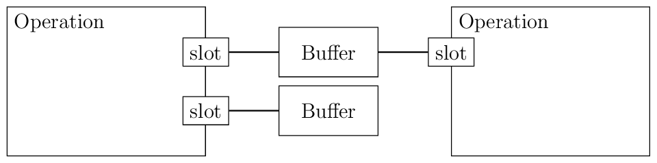
Visualization
As trees of operations get more complex it can become difficult to keep track
of how everything is connected. To help with this, one can use
visualize_operation() to generate a PDF showing a visualization of an
operation (refer to the documentation for how to use it). Here is what the
output looks like for the fill-reduce example above. The two shapes shown for
each buffer are the unpadded and padded shapes, which in this case happen to
be the same.